Next: Our implementation
Up: A quick guide to
Previous: A quick guide to
Wedgelet approximations were introduced by Donoho [1], as a
means to efficiently approximate piecewise constant images.
Generally speaking, these approximations are obtained by
partitioning the image domain adaptively into disjoint sets,
followed by computing an approximation of the image on each of
these sets. Optimal approximations are defined by means of a
certain functional weighing approximation error against complexity
of the decomposition. The optimization can be imagined as a game
of puzzle: The aim is to approximate the image by putting together
a number of pieces from a fixed set, possibly using a minimal
number of pieces.
As can be imagined, the efficient computation of such an optimal
approximation is a critical issue, depending on the particular
class of partitions under considerations. Donoho proposed to use
wedges, and to study the associated wedgelet approximations.
For the sake of notational convenience, we fix that images are
understood as elements of the function space  , where
 . Other image
sizes can be treated by suitable adaptation, at the cost of a more
complicated notation.
. Other image
sizes can be treated by suitable adaptation, at the cost of a more
complicated notation.
The wedgelet approach can be described by a two-step procedure:
- Decompose the image domain
 into a disjoint
union of wedge-shaped sets,
into a disjoint
union of wedge-shaped sets,
 .
.
- On each set
 , approximate the image by a
constant.
, approximate the image by a
constant.
Here the  are required to be elements of a
fixed set
are required to be elements of a
fixed set  of wedges.
A wedgelet
approximation of an image
of wedges.
A wedgelet
approximation of an image  associated to the regularization
parameter
associated to the regularization
parameter  is by definition a minimizer of the functional
 |
(1) |
Here  is a function which is constant on each wedge
, and
is a function which is constant on each wedge
, and  denotes the
  -norm on
,
-norm on
,
The
regularization parameter can be interpreted as a scale:
As ranges from  to
to  , the minimizer
 of (1) runs through a stack of
images, starting from the data (for
of (1) runs through a stack of
images, starting from the data (for  ) to a constant
image (for
) to a constant
image (for
 ).
).
A minimizer
 of
(1) can be viewed as an optimal approximation to
with a prescribed complexity: If
of
(1) can be viewed as an optimal approximation to
with a prescribed complexity: If
 , let
, let  denote the set of images in which
are constant on a partition of into at most
denote the set of images in which
are constant on a partition of into at most  wedges. Then
 is an element of with minimal
-distance to .
is an element of with minimal
-distance to .
A further useful observation is that since we consider constant
approximation,
is easily obtained from the
optimal partition
 by computing mean
values of over the elements of
. Hence the
minimization procedure boils down to finding the optimal
partition.
by computing mean
values of over the elements of
. Hence the
minimization procedure boils down to finding the optimal
partition.
This allows yet another interpretation of a minimizer
: Let
 . Then, among all wedge
partitions incurring an approximation error of at most
. Then, among all wedge
partitions incurring an approximation error of at most  ,
is the one with the smallest number of
elements.
,
is the one with the smallest number of
elements.
Hence, a minimization result of (1) can either be
viewed as optimal approximation with (at most) a fixed number
 of pieces, or as partition with a minimal number of
pieces among those partitions that incur (at most) a fixed
approximation error
of pieces, or as partition with a minimal number of
pieces among those partitions that incur (at most) a fixed
approximation error
 .
.
Clearly the properties of this scheme depend on the precise
definition of the set of admissible wedges. One
possible choice could be to take the set  of dyadic
squares contained in ,
of dyadic
squares contained in ,
Strictly speaking, the "wedges" appearing in this set do not
deserve the name, and approximations based on dyadic squares have
been studied for quite some time, usually under the name of
"quadtree decompositions". The wedgelet construction proposed by
Donoho can be seen as a refinement of this: Then elements of
are obtained by splitting an element
 along a suitable straight line, yielding
 . For
each dyadic square the lines are prescribed according to a
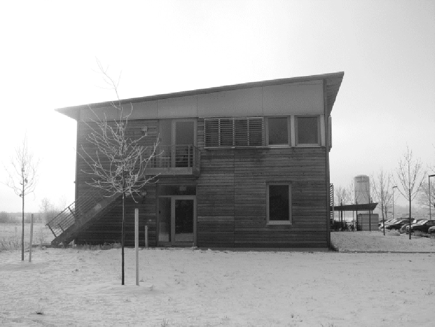
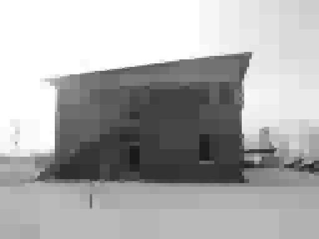
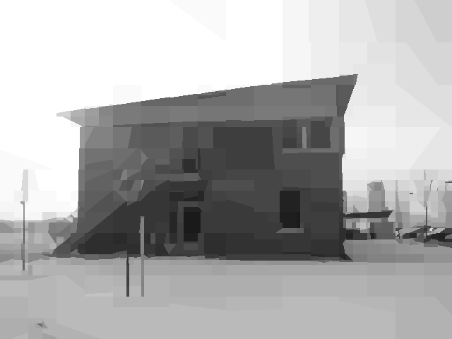
suitable scheme (more on that in the next section). Figure 1 shows
examples of optimal approximations using wedges and dyadic
squares, with the same number of pieces. Since coding wedges
requires more information per piece, the comparison is not exactly
fair; but the images manage to convey the motivation behind the
construction of wedgelets, which do a much better job at resolving
diagonal edges.
. For
each dyadic square the lines are prescribed according to a
suitable scheme (more on that in the next section). Figure 1 shows
examples of optimal approximations using wedges and dyadic
squares, with the same number of pieces. Since coding wedges
requires more information per piece, the comparison is not exactly
fair; but the images manage to convey the motivation behind the
construction of wedgelets, which do a much better job at resolving
diagonal edges.
Figure 1:
IBB North.
 (a) Original image, (b)
approximation using 1000 dyadic squares, and (c) approximation
using 1000 wedges.
(a) Original image, (b)
approximation using 1000 dyadic squares, and (c) approximation
using 1000 wedges.
|
|
With these definitions, an algorithm for the minimization of
(1) can be broken down into the following two steps:
- Local minimization: For each dyadic square, determine the wedge split
which yields the minimal local approximation error
 . Here
  is the restriction of to
  ,
and
,
and  is the function
that assigns each element of
is the function
that assigns each element of  the mean value of on
. Store the optimal split and associated approximation
error.
the mean value of on
. Store the optimal split and associated approximation
error.
- Global minimization: Given , compute the optimal wedgelet decomposition
 from the data stored in the first step.
This way of organizing the minimization procedure is based on the
following observations. We refer to [1,2] for more
details.
- From a computational point of view, local minimization
dominates the algorithm performance. We are required to compute
mean values and -errors for a large number of wedges, and
a naive approach to this problem results in huge computation
times. An effective solution of this problem is one of the main
contributions of our implementation.
- In view of the previous
remarks, it is important to note that the local minimization does
not depend on the parameter . The quadtree structure
associated to dyadic squares allows a fast implementation of the
global minimization step, yielding arbitrary access to the
minimizers of (1) almost in real time.
Next: Our implementation
Up: A quick guide to
Previous: A quick guide to
fof 050301